JUMP TO TOPIC

The concept of vertical intercept and its application to real-world scenarios is fundamentally the fascinating realm of mathematics. It provides an essential reference point in the graphical representation of linear equations, functions, and data trends.
This vital intersection point on the y-axis delivers invaluable insight into the inherent characteristics of the relationship described by the equation or function, enabling a comprehensive understanding of its behavior.
As we delve into the intricate world of the vertical intercept, we’ll explore its theoretical underpinnings, practical applications, and significance across diverse fields, including physics, economics, and engineering. This article promises to be enlightening, whether you’re a mathematics aficionado or a curious reader seeking to enhance your knowledge.
Defining the Vertical Intercept
The vertical intercept, often called the y-intercept, is critical in studying mathematical functions and their graphical representations. It is the point at which a line, curve, or surface intersects the vertical or y-axis on a Cartesian coordinate system.
In a two-dimensional graph representing a linear function, such as y = mx + b (where m is the slope and b is the y-intercept), the vertical intercept is the value of y when x equals zero (x = 0). This value is denoted by the constant term ‘b.’ Therefore, in this case, the vertical intercept provides the starting value of the function when the independent variable (x) has not yet influenced the outcome. Below is the representation of a generic vertical intercept for a linear function.
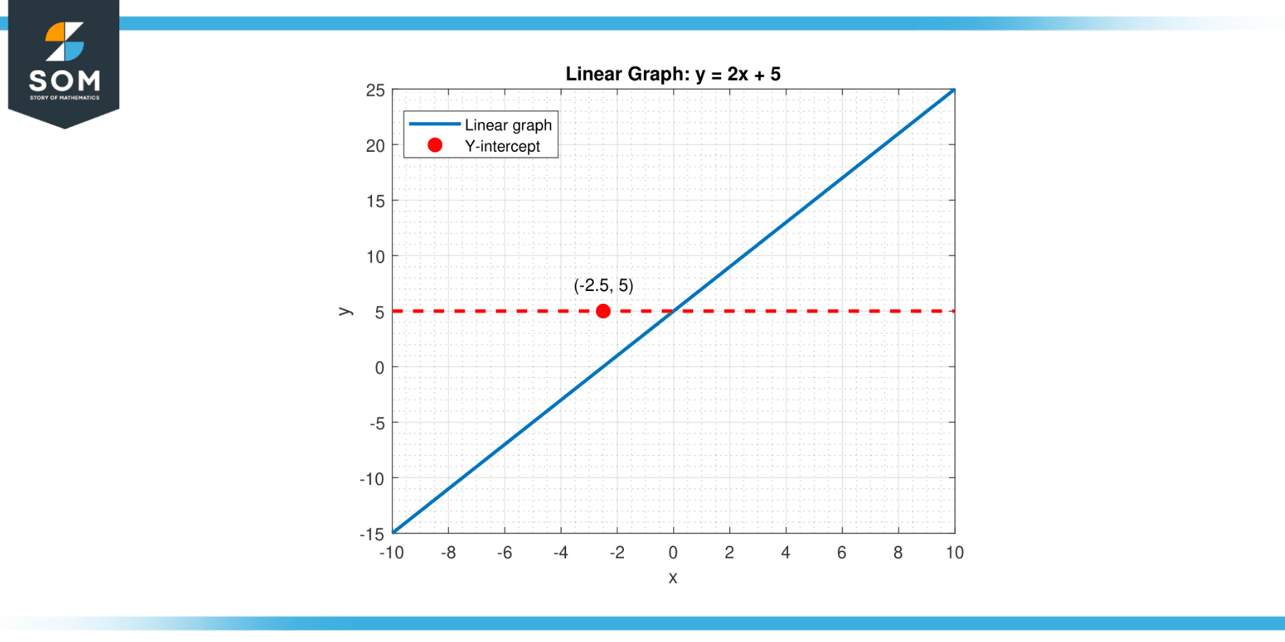
Figure-1.
For non-linear functions and curves, the concept is similar. The vertical intercept is still the point where the curve intersects the y-axis, marking the value of the function when the input or independent variable is zero. This fundamental concept forms the backbone of many analyses and problem-solving strategies in mathematics and various scientific and economic disciplines. Below is the representation of a generic vertical intercept for a non-linear function.
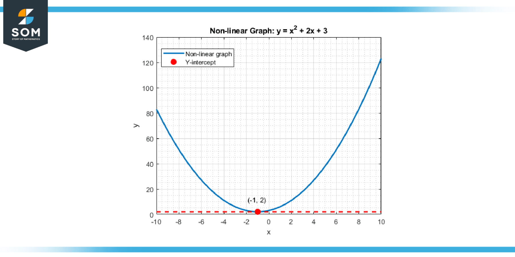
Figure-2.
Properties of Vertical Intercept
The vertical intercept is a foundational element in linear equations and mathematical functions. Its properties are closely related to the form and characteristics of the equation or function it represents. Here are some key properties:
Starting Point
In a real-world application, the vertical intercept often signifies a system’s starting point or initial condition before any changes are made. For example, in a business scenario, the vertical intercept of a cost function could represent the fixed costs before any units are produced.
Value at x = 0
The vertical intercept represents the value of the function when the independent variable, typically denoted as x, is zero. For instance, in the linear equation y = mx + b, when x = 0, y = b. Therefore, ‘b’ is the vertical intercept.
Graphical Intersection
The vertical intercept is the point where the graph of a function intersects the y-axis. This intersection is a valuable reference point in the graphical representation of functions and helps understand the function’s behavior.
Influence of Slope
For a linear function, the slope of the line doesn’t affect the vertical intercept. No matter how steep or shallow the line is, it does not change the point at which it crosses the y-axis.
Transformation Effects
The vertical intercept changes under vertical translations of the graph. If a constant is added or subtracted from the function (y = f(x) + c or y = f(x) – c), the graph shifts up or down, and this translates to a change in the vertical intercept.
Solving Equations
In a system of linear equations, the vertical intercept can be a crucial factor in solving the equations. If two lines have the same vertical intercept, they are either the same line (if they also have the same slope) or parallel lines (if they have different slopes).
These properties highlight the importance and versatility of the vertical intercept in various areas of mathematics and its applications. Whether you’re graphing a function, analyzing a real-world scenario, or solving a system of equations, the vertical intercept plays a significant role.
How to Find the Vertical Intercept
Finding the vertical intercept of a function involves setting the independent variable to zero and solving for the dependent variable. Here are the detailed steps:
Identify the Function
The first step in finding the vertical intercept is clearly understanding the function for which you seek the intercept. This could be a simple linear function such as y = mx + b, a quadratic function like y = ax² + bx + c, or a more complex non-linear function.
Set the Independent Variable to Zero
The vertical intercept is where the function crosses the y-axis, which happens when the independent variable (commonly x) equals zero. Therefore, you need to set x = 0 in the function. For instance, in the linear function y = mx + b, setting x = 0 gives y = b. So, ‘b’ is the vertical intercept.
Solve for the Dependent Variable
After setting the independent variable to zero, you solve the function for the dependent variable (commonly y). This gives you the y-coordinate of the vertical intercept. For example, in the quadratic function y = ax² + bx + c, setting x = 0 results in y = c. So, ‘c’ is the vertical intercept.
Determine the Coordinates of the Vertical Intercept
The vertical intercept is a point on the y-axis, so its x-coordinate is always zero. Pair this with the y-coordinate you found in the previous step, and you have the coordinates of the vertical intercept. For instance, if the y-coordinate is 5, the coordinates of the vertical intercept are (0, 5).
These steps apply to a wide range of functions, not only linear or quadratic functions. No matter how complex the function is, the vertical intercept is always found by setting the independent variable to zero and solving for the dependent variable.
Applications
The vertical intercept has wide-ranging applications across various fields of study. Its importance goes far beyond merely identifying a point on a graph; it often offers a practical interpretation or starting point for a process or phenomenon. Here are a few examples:
Economics and Business
In economics, linear models are often used to represent cost, revenue, and profit functions. The vertical intercept in these functions typically represents a base or fixed cost that doesn’t depend on the output level. For instance, in a cost function C = mx + b, where m is the variable cost per unit and x is the number of units produced, the vertical intercept ‘b’ represents the fixed costs that must be paid regardless of production levels.
Physics
In physics, the vertical intercept can represent initial conditions in a motion problem. For example, in the equation for simple harmonic motion or the trajectory of a projectile, the vertical intercept may represent an object’s initial position or height.
Environmental Science
In modeling population growth or decay of pollutants, the vertical intercept can represent a substance’s initial population size or quantity.
Chemistry
In the equation for a reaction rate, the vertical intercept can represent the initial concentration of a reactant.
Engineering
In stress-strain graphs, the vertical intercept represents the proportional limit. Beyond this point, the material will no longer return to its original shape when the stress is removed.
Statistics and Data Analysis
In regression analysis, the vertical intercept represents the expected value of the dependent variable when all independent variables are zero. This can provide a baseline for comparison when evaluating the effects of different variables.
In all these fields and many others, understanding the significance of the vertical intercept enables a more meaningful interpretation of mathematical models and their real-world implications.
Exercise
Example 1
Consider the linear function y = 2x + 3, and find the vertical intercept.
Solution
The vertical intercept can be found by setting x = 0:
y = 2(0) + 3
y = 3
So, the vertical intercept of the function is the point (0, 3).
Example 2
Consider the quadratic function y = -x² + 5x – 4, as given in Figure-3, and find the vertical intercept.
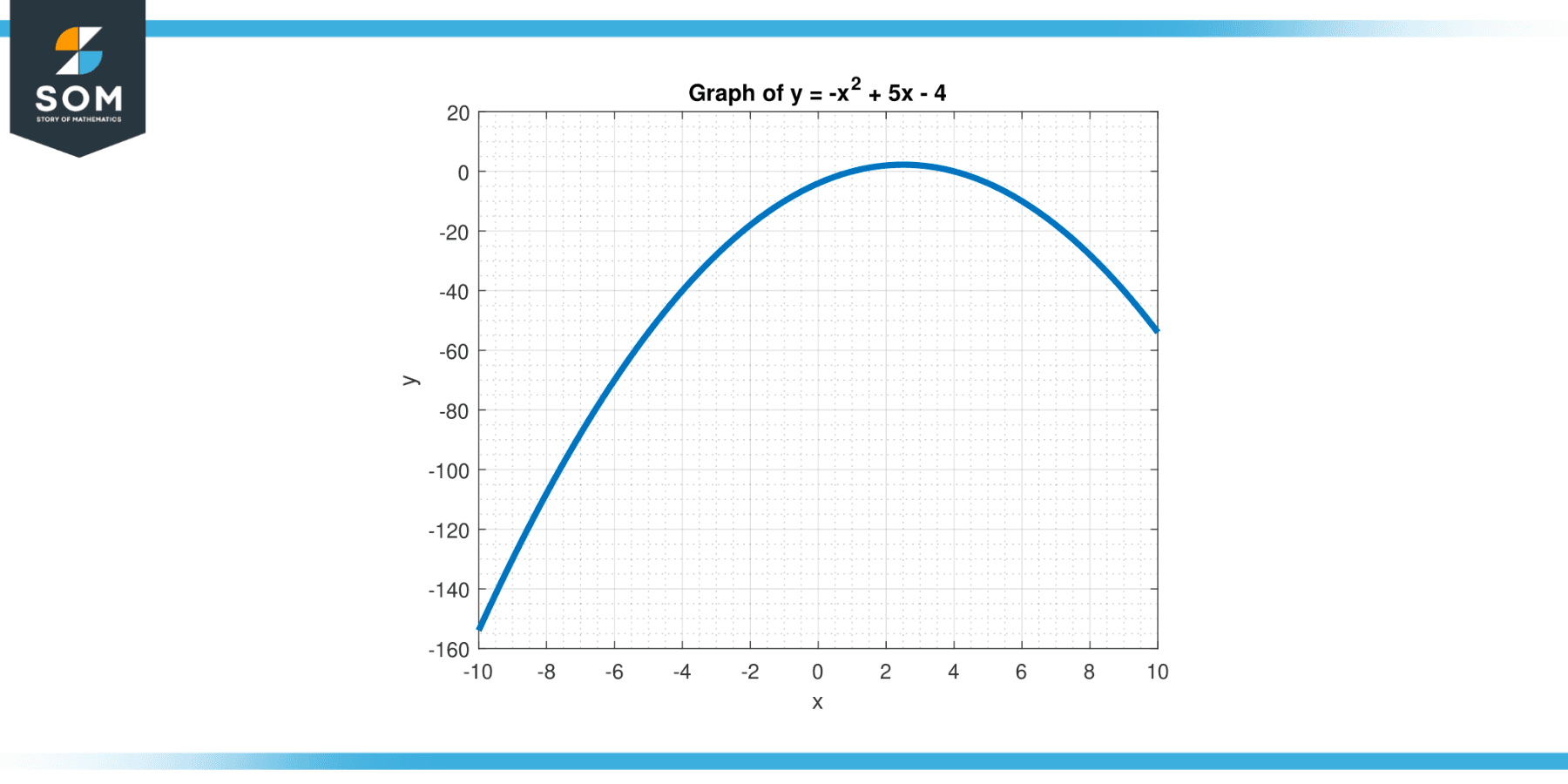
Figure-3.
Solution
The vertical intercept is found by setting x = 0:
y = -0² + 5(0) – 4
y = -4
The vertical intercept of this function is the point (0, -4).
Example 3
Consider the cubic function y = x³ – 2x² + x, and find the vertical intercept.
Solution
The vertical intercept is found by setting x = 0:
y = 0³ – 2*0² + 0
y = 0
So, the vertical intercept of this function is the point (0, 0).
Example 4
Calculate the verticle intercept for the function y = 3 * $e^{2x}$, as given in Figure-4.
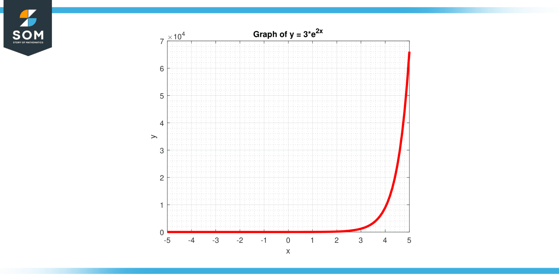
Figure-4.
Solution
The vertical intercept is found by setting x = 0:
y = 3 * $e^{2x}$
y = 3
The vertical intercept of this function is the point (0, 3).
Example 5
Consider the function y = (1/2)log(x) + 3, and find the verticle intercept.
Solution
Even though we usually find the vertical intercept by setting x = 0, the domain of the logarithm function is x > 0, so this function does not have a vertical intercept.
Example 6
Consider the function y = -$2^{x}$ + 5, as given in Figure-5, and find the verticle intercept.
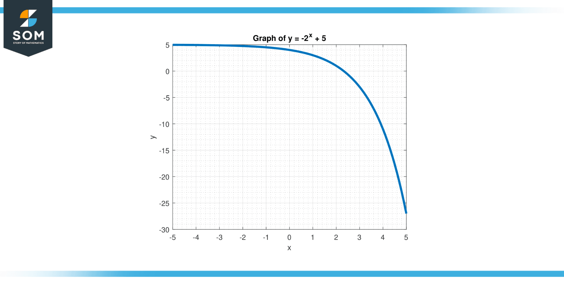
Figure-5.
Solution
The vertical intercept is found by setting x = 0:
y = -$2^{0}$ + 5
y = -1 + 5
y = 4
So, the vertical intercept of this function is the point (0, 4).
Example 7
Consider the function y = 4/(x-3) + 2, and find the verticle intercept
Solution
Even though we usually find the vertical intercept by setting x = 0, x cannot be 3 for this function because it would make the denominator 0. But when x = 0, we find:
y = 4/(0-3) + 2
y = -4/3 + 2
y = -4/3 + 6/3
y = 2/3
So, the vertical intercept of this function is the point (0, 2/3).
Example 8
Consider the function y = (3x – 2) / (x + 1), and find the verticle intercept
Solution
The vertical intercept is found by setting x = 0:
y = (3 * 0 – 2) / (0 + 1)
y = -2 / 1
y = -2
The vertical intercept of this function is the point (0, -2).
All figures are generated using MATLAB.
