JUMP TO TOPIC
Piecewise Laplace Transform + Online Solver With Free Steps
A piecewise Laplace transform calculator is a calculator used to find out the s-domain complex solution for a piecewise time domain signal which is not continuous at some point in time, and thus exists in more than one definition.
Where the solution of this piecewise function is expressed in the proper s-domain format once the Laplace transform is applied, for any 2-piecewise time-domain function.
What Is a Piecewise Laplace Transform Calculator?
A Piecewise Laplace Transform Calculator is an online tool that is used for finding the Laplace transforms of complex functions quickly which require a lot of time if done manually.
A standard time-domain function can easily be converted into an s-domain signal using a plain old Laplace transform. But when it comes to solving a function that has more than one part associated with it i.e., a piecewise time-domain function, only this calculator can help you. As it can, not only patch together the pieces of such a piecewise time-domain function but also can calculate a singular s-domain Laplace transform for it.

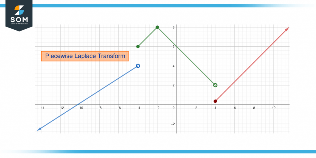
Figure 1: Piecewise Functions
Now to utilize its functionalities, you may first require a piecewise function, with both its definition and the intervals for which, each is valid. Once you have all that, you can enter those values inside the input boxes given in the calculator’s interface.
How To Use the Piecewise Laplace Transform Calculator?
Piecewise Laplace Transform calculator is very easy to use if you have all the required values and thus, following the given steps will ensure that you get the result that you desire from this calculator. So, to find
the Laplace transform of a piecewise function you may proceed as follows.
Step 1:
Use the calculator to calculate the Laplace transform of the desired function.
Step 2:
Enter the piecewise time-domain function into the given input boxes. One must understand that this calculator is equipped with functionalities that allow it to only solve functions with a maximum of one discontinuity which means, that it can only allow two pieces of a function.
Step 3:
Now, you may enter the intervals provided for each of the piecewise function’s parts given to you. This represents the time interval for the part on each side of the discontinuity.
Step 4:
Lastly, you just click on the button “Submit” and it will open the whole step-by-step solution of the piecewise time-domain function starting from the conversion to the s-domain, leading up to the final Laplace transform simplified notation.
As we have mentioned before that this calculator can only solve for one discontinuity carrying piecewise function. And it’s beneficial to notice that usually the given piecewise functions very rarely would ever go above having 2 discontinuities, thus 3-parts. And most of the time, one of these 3-parts would represent a zero output. And under those circumstances, the zero output can easily be neglected to get a viable solution to the problem.
How Does a Piecewise Laplace Transform Calculator Work?

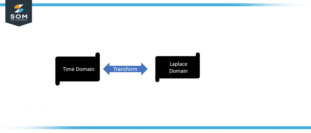
Figure-1 Laplace Transform
Let’s figure out how a Laplace Transform Calculator works.
The Laplace transform calculator works by solving complex functions quickly without any hassle. It shows the result generated in the following forms:
- It shows the input as an Ordinary Differential Equation (ODE).
- Secondly, it explains the answer in algebraic form.
- The Laplace transform calculator can also give you detailed steps of the solution if you want.
Now, let’s have a brief insight into some important concepts.
What Is a Laplace Transform?
A Laplace Transform is an integral transform that is used to convert a time-domain function into an s-domain signal. And this is done because a time-domain differential function is often very difficult to extract information from. A Laplace transform is an integral transform that is used to convert a time-domain function into an s- domain signal.
But, once in the s-domain, it becomes very easy to navigate through as it can all be represented in terms of a polynomial and this Laplace transformation can be carried out using a set of principles that have been laid out by mathematicians. These can also be found in a Laplace table.
What Is a Piecewise Function?
A piecewise function is a function that represents a time-domain function with inequality at a certain point in time in the output of the function. In a real mathematical scenario, it is very clear that a function cannot have two different values at the same time. This is why this type of function is expressed with a discontinuity.
Hence, the best way to handle such a problem is to divide this function into subparts because there is no correlation in the outputs of these two pieces at the point of discontinuity and onwards, and thus a piecewise function is born.
How To Take the Laplace Transform Of a Piecewise Function?
In order to take a Laplace transforms onto a piecewise function in the time domain, following the standard method that relies on taking both pieces of the input function and applying convolution to them, as their outputs don’t correlate for every value in their intervals.
Therefore, adding the impulse responses of each piece together, and getting a singular impulse response of the overall function with the appropriate limits is the best way to go about things.
This is then made to go through a Laplace transform using the rules of the Laplacian and a solution is derived that is finally simplified and expressed.
This is how the Laplace Transform calculator for a piecewise function calculates its
solutions.
Solved Examples:
Example No.1:
Consider the following function:
\[ f(t) = \left\{\begin{array}{ll}t-1 & \quad 1 \leq t < 2 \\t+1 & \quad t > 2\end{array}\right\}(s)\]
Calculate the Laplace Transform using the calculator.
Now, the solution to this problem is as follows.
First, the Input can be interpreted as the Laplacian of the piecewise function:
\begin{equation*}
\mathcal{L} \bigg[\left\{
\begin{array}{ll}
t-1 & \quad 1 \leq t < 2 \\ t+1 & \quad t > 2
\end{array}
\right\}(s)\bigg]
\end{equation*}
The result is given after the Laplace Transform is applied:
\[ \dfrac{e^{-2s}(2s + e^s)}{s^2} \]
An alternate form can also be expressed as,
\[
\begin{align*}
\left \{\dfrac{2e^{-2s}s + e^{-s}}{s^2}\right\} \end{align*} \]
The final form of the results is given as:
\[ \begin{align*}
\left \{\dfrac{e^{-s}}{s^2}\right\} + \left \{\dfrac{2e^{-2s}}{s}\right\} \end{align*} \]
So, the result was mainly found in the first step when in the backend the combined impulse
response of the piecewise function had been converted to an s-domain, after that it was only a matter of simplification.
Example No.2:
Consider the following function:
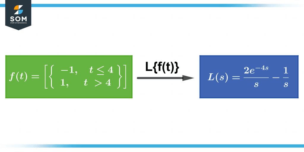
\[ f(t) = \left\{\begin{array}{ll}-1, \quad t \leq 4 \\1, \quad t>4\end{array}\right\}(s)\]
Calculate its Laplace Transform using the Laplace transform Calculator.
Now, the solution to this problem is as follows.
First, the Input can be interpreted as the Laplacian of the piecewise function:
\begin{equation*}
\mathcal{L} \bigg[\left\{
\begin{array}{ll}
-1, \quad t \leq 4 \\
1, \quad t > 4
\end{array}
\right\}(s)\bigg]
\end{equation*}
The result is given after the Laplace Transform is applied:
\[ \dfrac{ 2e^{-4s} – 1}{s} \]

Figure 3: Laplace Transform
An alternate form can also be expressed as:
\[ -\dfrac{e^{-4s}(e^{4s}-2}{s} \]
The final form of the results is given below:
\[ \dfrac{2e^{-4s}}{s} – \dfrac{1}{s} \]
So, the result was mainly found in the first step when in the backend the combined impulse
response of the piecewise function had been converted to an s-domain, after that it was only a matter of simplification.
