JUMP TO TOPIC

Within the world of calculus, we explore the derivative of x² through applications and examples that help us make sense of the myriad phenomena in science and engineering. The derivative is a tool that helps us understand rates of change and slopes of curves. A classic and instructive example is the derivative of x², a simple parabolic function.
In this article, we will delve deep into understanding the derivative of x², its computation, and the fundamental insights it provides into the function’s behavior. From the realms of pure mathematics to physics and engineering, this derivative holds a key place, demonstrating the quintessential nature of calculus in our comprehension of the universe.
Defining Derivative of x²
The derivative of a function quantifies the rate at which the output of the function changes with respect to changes in its input. In the context of x², its derivative provides the rate of change of the square of x with respect to x itself.
Mathematically, the derivative of a function f(x) at a specific point x is defined as the limit as Δx approaches 0 of the difference quotient [f(x + Δx) – f(x)]/Δx. Applying this to the function f(x) = x², we find that the derivative, often denoted as f'(x) or df(x)/dx, equals 2x.
As a result, any point x on the curve will be true. y = x², the rate of change at that point is 2x. Hence, the derivative of the function x² gives provides us the slope of the curve’s tangent line y = x² at any point (x, x²) on the curve.
This result is fundamental in the calculus and has significant implications in various fields, such as physics, economics, and engineering, where understanding the rate of change of quantities is crucial.
Graphical Representation of Derivative of x²
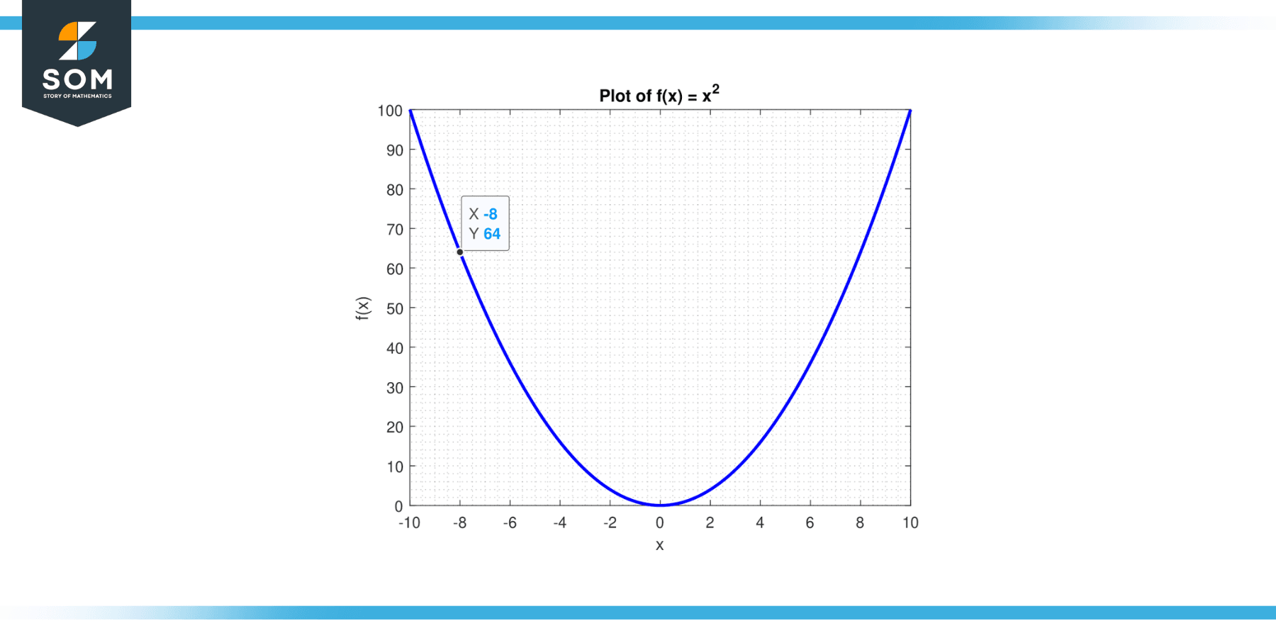
The function f(x) = x² is a simple parabolic function, which graphically represents a parabola opening upwards with its vertex at the origin (0, 0). The result of taking this function’s derivative is f'(x) = 2x. Below we present the graphical representation of the function f(x) = x² in Figure-1.

Figure-1.
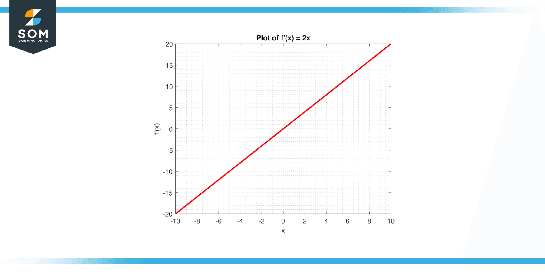
Graphically, the function f'(x) = 2x is a straight line that passes through the origin. The slope of this line is 2, indicating that for each unit increase in x, the function value increases by 2 units. This line cuts the x-axis at the origin and divides the plane into two halves, with the function being positive in the right half (for x > 0) and negative in the left half (for x < 0). Below we present the graphical representation of the function f'(x) = 2x in Figure-2.

Figure-2.
Moreover, the function f'(x) = 2x represents the angle at which the curve’s tangent line slopes y = x² at any point (x, x²) on the curve. When x = 0, the derivative is also 0, indicating a horizontal tangent at the vertex of the parabola y = x². As the x-axis is extended away from the origin, the value of the derivative increases or decreases linearly.
This corresponds to the parabola y = x² getting steeper as we move away from the vertex in either direction and the angle at which the tangent line to the curve slopes matches the value of the derivative at that point.
Properties
The derivative of the function f(x) = x² is f'(x) = 2x, and it possesses several key properties that emerge from the fundamental principles of calculus.
Linearity
This is a critical property of all derivatives, not just the derivative of x². It indicates that the derivative of a constant times a function is the same as the derivative of the constant times the function, and the derivative of a constant times the product of two functions equals the total of the derivatives of the two functions. If we consider a function g(x) = ax² + bx (where a and b are constants), its derivative would be g'(x) = 2ax + b, demonstrating the linearity property.
Increasing Function
The derivative f'(x) = 2x is an increasing function. This means that as x increases, the value of 2x also increases. Therefore, the slope of the tangent line to the curve y = x² increases as we move from left to right along the curve. This reflects the fundamental property of the parabola y = x², which gets steeper as we move away from its vertex.
Slope of Tangent
The derivative of x² at a given point provides the slope of the tangent to the curve y = x² at that point. For example, if we take x = 3, then the derivative f'(3) = 2*3 = 6. This reveals that the point’s tangent line’s slope to the curve (3, 9) is 6.
Instantaneous Rate of Change
The derivative f'(x) = 2x represents the instantaneous rate of change of y = x² with respect to x. That is, it shows how rapidly the square of a number changes as the number itself changes.
Null at Origin
The derivative of x² is zero when x = 0, meaning there is a horizontal tangent to the curve y = x² at the origin. This corresponds to the fact that the function x² reaches a minimum value at x = 0.
Symmetry
The derivative f'(x) = 2x is a symmetric function with respect to the origin since it is an odd function. This aligns with the fact that the function x² and its derivative share the same symmetry axis, the y-axis.
By understanding these properties, one gains a deeper comprehension of the derivative of x² and how it reflects the characteristics of the function it is derived from. This understanding is also fundamental to applying calculus in solving real-world problems.
Applications
The derivative of the function x² plays a crucial role in several fields, often where the concept of change, growth, or rates is essential. Below, we’ve highlighted its applications in a few different areas:
Physics
In physics, the derivative of x² frequently arises when dealing with motion. A function of time can frequently be used to represent the position of an item travelling down a line. If an object’s location is indicated by s(t) = t², its velocity, which is the derivative of the position function, is given by v(t) = 2t. This tells us how fast the object is moving at any instant.
Economics
In economics, derivatives are used to model cost functions. As an illustration, if the whole cost of production x units is given by C(x) = x², the derivative, C'(x) = 2x, indicates the cost of producing one additional unit, or the marginal cost. This information is invaluable in deciding production levels to maximize profits.
Engineering
In various branches of engineering, the derivative of x² has applications in optimization problems, control systems, and modeling physical systems. For example, if the signal strength of a transmitter varies as the square of the distance from it, understanding the rate of change of signal strength can be crucial in designing efficient communication systems.
Computer Graphics
In computer graphics, the derivative of curves, like the parabola x², is used for rendering and animation. By understanding how the curve changes at each point (its derivative), graphics software can create smooth and realistic representations of objects and motion.
Biology
In biology, the derivative of x² can be used in population models where a population’s growth rate is proportional to the size of the population itself.
Environmental Science
In environmental science, such concepts may be used in pollutant spread or heat distribution models, where rates of change are crucial for understanding and predicting outcomes.
In all these fields, the fundamental idea is the same: the derivative of a function, including x², gives us an understanding of how a quantity changes in response to changes in input. This is a powerful concept with broad applicability across disciplines.
Exercise
Example 1
What is the tangent line’s slope to the curve, y = x² at the point (2,4)?
Solution
To determine the slope of the curve’s tangent line at a specific location, we take the derivative of the function and evaluate it at the given x-coordinate. The derivative of y = x² is:
y’ = 2x
To find the slope at point (2,4), we substitute x = 2 into the derivative, yielding:
y'(2) = 2 * 2
y'(2) = 4
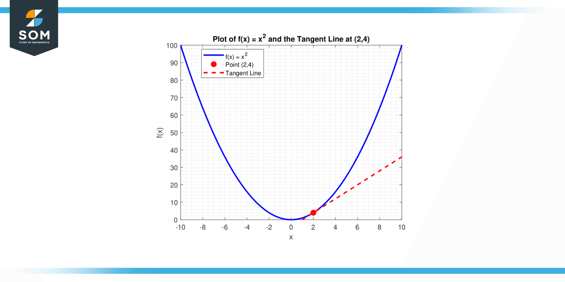
Consequently, the angle between the tangent line to the curve and the point (2,4) is 4. Below we present the same in graphical form.

Figure-3.
Example 2
At what points on the curve y = x² does the tangent line pass through the origin?
Solution
A line that passes through the origin has the equation y = mx, where m is the slope of the line. If the tangent line to the curve y = x² passes through the origin, its slope at the point (x, x²) must be x because the line connects (x, x²) and (0, 0). Therefore, we set the derivative equal to x:
2x = x
Solving this equation gives us x = 0, indicating that the only point on the curve y = x² where the tangent line passes through the origin is at (0,0).
Example 3
What is the tangent line’s slope to the curve, y = x² at the point (3, 9)?
Solution
To determine the slope of the curve’s tangent line at a specific location, we first find the function’s derivative to determine the tangent line’s slope. The derivative of y = x² is:
y’ = 2x
The slope of the tangent line at x = 3 is thus:
y'(3) = 2 * 3
y'(3) = 6
A line with slope m passing through a point (x₁, y₁) has the equation y – y₁ = m(x – x₁). Substituting m = 6 and (x₁, y₁) = (3, 9) gives us:
y – 9 = 6(x – 3)
or equivalently:
y = 6x – 9
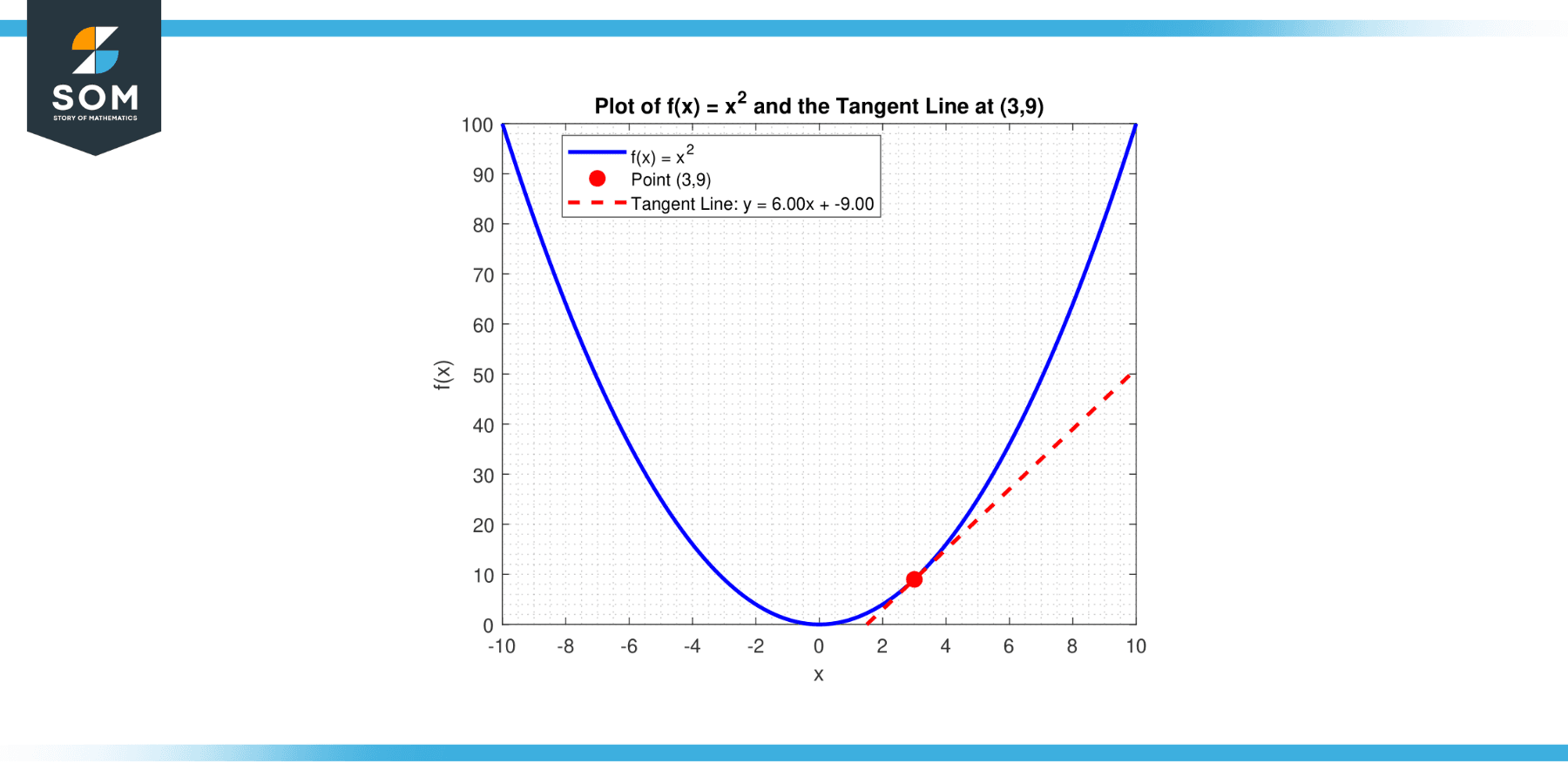
Below we present the same in graphical form.

Figure-4.
Example 4
Suppose a particle is moving along a line such that its position at any time t (in seconds) is given by s(t) = t² (in meters).What is the particle’s speed at? t = 3 seconds?
Solution
Here, the particle’s velocity is the derivative of the position function. The derivative of s(t) = t² is:
s'(t) = 2t
So, the velocity at t = 3 is:
s'(3) = 2*3
s'(3) = 6 meters per second
Example 5
Suppose a company’s total cost C (in dollars) of producing x units of a product is given by C(x) = 500x². What is the marginal cost when x = 100?
Solution
The marginal cost is the rate of change of the total cost with respect to the number of units produced, i.e., it’s the derivative of the cost function. The derivative of C(x) = 500x² is:
C'(x) = 1000x
Therefore, the marginal cost at x = 100 is:
C'(100) = 1000*100
C'(100) = $100,000 per unit
All images were created with MATLAB.
